Looking for IGNOU MMPC-010 Managerial Economics solved assignment 2026? This page provides complete, well-structured and easy-to-understand answers for the MMPC-010 TMA/Assignment, covering all the questions from the current assignment. Use these answers as a reference to understand key concepts such as Equi-Marginal Principle, Price Elasticity of Demand, Isoquants, Isocost, Perfect Competition, Monopoly and Price Discrimination.

QUESTION 1:
The Equi-Marginal Principle can be applied to both consumption as well as production”. Discuss this statement with the help of an example.
The Equi-Marginal Principle, also known as the Law of Equi-Marginal Utility or the Law of Substitution, is an important principle of economics that explains how a rational individual or firm allocates scarce resources among competing uses. Since resources such as income, time, labour, capital and raw materials are limited, they must be allocated in such a way that the maximum possible satisfaction or output is obtained.
The principle states that a consumer or producer achieves an optimum allocation of resources when the marginal benefit obtained from the last unit of resource used in each alternative is equal. In simple words, a person should continue transferring resources from a use where the marginal return is relatively low to a use where the marginal return is relatively high. This process continues until the returns from the different uses become equal, subject to the relevant prices and constraints.
The principle can therefore be expressed as:
Marginal Benefit per Unit of Resource = Equal across alternative uses
The basic idea is that a scarce resource should not remain allocated to a low-return activity when it can produce a higher return elsewhere. The principle is applicable mainly in two important areas: consumption and production.
Application in Consumption
In the theory of consumer behaviour, the Equi-Marginal Principle is expressed as the Law of Equi-Marginal Utility. A consumer has limited income but may have many goods and services from which to choose. Therefore, the consumer has to distribute income among different goods in such a way that total satisfaction is maximised.
According to this principle, a consumer reaches equilibrium when the marginal utility obtained per rupee spent on each commodity is equal. For two commodities X and Y, the condition can be expressed as:
MUx / Px = MUy / Py = Marginal Utility of Money
Where:
- MUx = Marginal utility of commodity X
- MUy = Marginal utility of commodity Y
- Px = Price of commodity X
- Py = Price of commodity Y
This condition means that the last rupee spent on each commodity should provide the same amount of additional satisfaction.
If:
MUx / Px > MUy / Py
the consumer receives greater satisfaction from spending an additional rupee on X than on Y. Therefore, the consumer should spend more on X and less on Y. As more units of X are consumed, its marginal utility generally decreases because of the Law of Diminishing Marginal Utility. At the same time, reducing expenditure on Y can change its marginal utility. The consumer continues this process until the marginal utility per rupee becomes equal for both commodities.
Example of Consumption
Suppose a student has ₹100 to spend on tea and samosas. Assume that both tea and samosas cost ₹10 each.
If the marginal utility of the fourth cup of tea is 40 utils, then:
MU of tea / Price of tea = 40 / 10 = 4 utils per rupee
If the marginal utility of the fourth samosa is 60 utils, then:
MU of samosa / Price of samosa = 60 / 10 = 6 utils per rupee
Since 6 utils per rupee from samosas is greater than 4 utils per rupee from tea, the student should allocate more expenditure towards samosas and relatively less towards tea.
As the student consumes more samosas, their marginal utility is expected to decline. Eventually, a point may be reached where:
MU of tea / Price of tea = MU of samosa / Price of samosa
For example:
IGNOU MMPC-008 Solved Assignment 2026 | Easy & Accurate Answers
IGNOU MMPC-009 Solved Assignment 2026 | Easy & Accurate Answers
50 / ₹10 = 50 / ₹10 = 5 utils per rupee
At this point, there is no advantage in shifting another rupee from one commodity to the other. The consumer has achieved maximum total utility from the available income.
Thus, the Equi-Marginal Principle helps explain how a consumer can obtain maximum satisfaction from a limited income.
Application in Production
The Equi-Marginal Principle is also applicable to the production decisions of a firm. A producer has limited resources such as labour, capital, machinery, raw materials and finance. These resources can be used in different combinations and activities. The producer therefore needs to allocate resources efficiently to obtain maximum output or minimise the cost of producing a given level of output.
In production theory, the principle is associated with the Law of Equi-Marginal Returns and the least-cost combination of inputs.
Suppose a firm uses two inputs, labour (L) and capital (K). The firm reaches an optimum allocation when the marginal product obtained from the last rupee spent on labour is equal to the marginal product obtained from the last rupee spent on capital.
The condition can be written as:
MPL / w = MPK / r
Where:
- MPL = Marginal Product of Labour
- MPK = Marginal Product of Capital
- w = Wage rate of labour
- r = Rental price or cost of capital
This means that the firm should compare the additional output obtained from every rupee spent on different inputs.
If:
MPL / w > MPK / r
labour is producing more output per rupee than capital. The firm should therefore increase its expenditure on labour and reduce its expenditure on capital, subject to its production and budget constraints.
Similarly, if:
MPK / r > MPL / w
the firm should allocate relatively more resources to capital.
The adjustment continues until:
MPL / w = MPK / r
At this point, the firm cannot increase output further by simply transferring expenditure from one input to another. The available resources have been allocated efficiently.
Example of Production
Consider a garment factory with a fixed monthly production budget. The factory can use the budget to employ additional workers or obtain additional machine hours.
Suppose:
- One additional ₹1,000 spent on labour produces 80 additional shirts.
- One additional ₹1,000 spent on machinery produces 50 additional shirts.
The marginal product per rupee is therefore higher for labour. The firm should initially allocate more of its budget towards labour.
As more labour is employed, the marginal product of labour may decline because of diminishing marginal returns. At the same time, reducing the use of machinery can make additional machine capacity relatively more valuable.
The firm should continue reallocating expenditure until the output obtained from the last rupee spent on labour becomes equal to the output obtained from the last rupee spent on capital.
Thus:
MPL / w = MPK / r
At this point, the firm has reached an efficient allocation of its limited production budget.
Application to Allocation Among Different Activities
The Equi-Marginal Principle can also be applied when a firm has to distribute a limited budget among different products, projects or business activities.
For example, suppose a company has ₹10 lakh available for investment in two projects. If the marginal return from the last rupee invested in Project A is higher than that from Project B, the company should shift some investment towards Project A. As additional resources are allocated to Project A, its marginal return may decline. The process continues until the marginal return per rupee is equalised across the alternative investments.
Therefore, the principle provides a general rule for the efficient allocation of scarce resources.
Importance of the Equi-Marginal Principle
The principle is important because it helps economic agents make rational decisions under conditions of scarcity.
- Maximum satisfaction: It helps consumers allocate limited income to obtain maximum total utility.
- Efficient use of resources: It ensures that scarce resources are directed towards their most productive uses.
- Cost minimisation: Producers can select an appropriate combination of inputs to produce output at minimum cost.
- Output maximisation: A firm can distribute its available resources in a way that maximises production.
- Investment decisions: Businesses can allocate limited funds among alternative projects according to their marginal returns.
- Resource substitution: It provides a basis for shifting resources from relatively less productive uses to more productive uses.
EXAMPLE : A restaurant has a fixed monthly budget for improving its kitchen. It can spend the money on hiring additional kitchen staff or purchasing additional cooking equipment. Initially, if spending ₹1,000 on an additional worker helps the restaurant prepare 8 extra meals, while ₹1,000 spent on equipment helps prepare only 5 extra meals, the restaurant will allocate more of its budget to labour. As more workers are hired, the additional output from each new worker may gradually fall because the kitchen becomes crowded. At the same time, the marginal benefit from additional equipment may increase. The restaurant will continue adjusting its spending until the additional output obtained from the last rupee spent on labour is equal to that obtained from the last rupee spent on equipment. This illustrates the Equi-Marginal Principle in a real-life business situation.
Conclusion
The Equi-Marginal Principle is thus a unifying rule of rational choice under scarcity: whether the scarce resource is a consumer’s income or a producer’s input budget, optimum allocation requires that the marginal return per unit of the scarce resource be equal across all competing uses. It formalises the common-sense idea of ‘not putting all eggs in one basket’ and reallocating resources towards their most productive uses until returns are balanced at the margin.
Q2. “The main determinant of elasticity is the availability of substitutes.” Explain this statement in the context of Price elasticity of demand.
Price elasticity of demand (Ped) measures the responsiveness of quantity demanded to a change in price: Ped = (% change in quantity demanded) / (% change in price). Demand is called elastic when Ped is numerically greater than 1 (quantity responds more than proportionately to price), inelastic when Ped is less than 1 (quantity responds less than proportionately), and unitary when Ped equals 1. While several factors influence elasticity — the nature of the good (necessity vs luxury), proportion of income spent on it, time period, and habit formation — the availability of close substitutes is widely regarded as the single most powerful determinant, because it directly governs how easily a consumer can escape a price increase.
Why Substitutes Matter So Much
When close substitutes are readily available, consumers can easily switch away from a good whose price rises, so demand for that good is highly elastic. Conversely, when a good has few or no substitutes, consumers have little choice but to continue buying it even at a higher price, making demand inelastic. The logic follows directly from the definition of a substitute: the cross-price elasticity between the good and its substitute is positive, and the more responsive consumers are to that cross-price relationship, the more elastic the original good’s own-price demand becomes.
This can be seen formally. Suppose good X has a close substitute Y. When Px rises, two forces act on the quantity demanded of X: the income effect (the consumer’s real purchasing power falls) and the substitution effect (X becomes relatively more expensive than Y, so consumers switch toward Y). The stronger and more available the substitute, the larger the substitution effect, and since the substitution effect is what makes demand curves slope downward sharply, availability of substitutes becomes the dominant force behind the size of Ped. At the theoretical extreme, if a good had a perfect substitute available at an unchanged price, its own demand curve would become perfectly (infinitely) elastic — the slightest price rise would cause quantity demanded to fall to zero as buyers switch entirely to the substitute. At the other extreme, a good with literally no substitute (a good on which survival depends, with no alternative source) would have a demand curve approaching perfect inelasticity, where quantity demanded barely changes regardless of price.
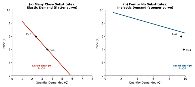
Figure: A flatter demand curve (panel a) reflects the presence of many close substitutes — a small price change produces a large change in quantity demanded. A steeper curve (panel b) reflects few or no substitutes — even a large price change produces only a small change in quantity demanded.
Illustrations
- Branded goods vs generic categories: The demand for a specific brand of soft drink (e.g., one particular cola) is highly elastic because rival colas and other beverages are close substitutes — a price rise induces consumers to switch brands. However, the demand for the broad category ‘soft drinks’ as a whole is far less elastic because the substitutes available (tea, juice, water) are more distant.
- Necessities with no substitutes: Life-saving medicines, salt, or electricity for essential household use have very few substitutes, so their demand is inelastic — consumers continue purchasing them even when prices rise.
- Goods with many alternatives: Consumer durables like televisions of different brands, or transport options like bus/train/cab for a given route, have many substitutes, making demand for any one option quite elastic.
- Narrow vs broad market definition: The narrower the definition of a commodity, the more substitutes it has and the more elastic its demand. ‘Apples’ has more substitutes (oranges, bananas) than ‘fruit’ in general, whose substitutes are far fewer, so demand for a specific fruit is more elastic than demand for fruit as a category.
- Fuel and transport: Petrol for private vehicles has traditionally shown inelastic demand in the short run because commuters have few immediate substitutes for a journey they must make; but where a good public transport network (bus, metro) exists as a genuine substitute, demand for petrol becomes noticeably more elastic, since commuters can shift mode of travel.
- Habit-forming and addictive goods: Cigarettes and tobacco products are a classic example of an inelastic good precisely because addiction reduces the practical substitutability of any alternative in the consumer’s mind, even though other goods physically exist in the market. This shows that ‘substitutes’ must be understood as substitutes from the consumer’s subjective perspective, not merely items that an economist might classify as similar.
Illustrative Elasticity Estimates
The pattern predicted by theory is broadly confirmed by empirically estimated elasticities for different categories of goods, summarised below. Goods towards the top of the table have abundant substitutes and show high (elastic) coefficients; goods towards the bottom have few substitutes and show low (inelastic) coefficients. (Figures are illustrative, representative orders of magnitude commonly cited in economics texts rather than estimates for any single country or year.)
| Good/Service | Typical availability of substitutes | Approximate Ped | Elastic / Inelastic |
| Restaurant meals out | Very high (many eateries, home cooking) | ≈ 2.3 | Highly elastic |
| A specific branded soft drink | High (rival brands, other beverages) | ≈ 1.5 – 2.0 | Elastic |
| Air travel (leisure) | Moderate–high (rail, bus, deferring trip) | ≈ 1.2 – 1.5 | Elastic |
| Housing (broad category) | Low–moderate (location-specific) | ≈ 0.6 – 0.9 | Inelastic |
| Cigarettes/tobacco | Very low (habit/addiction) | ≈ 0.3 – 0.5 | Inelastic |
| Salt | Almost none | ≈ 0.1 | Highly inelastic |
| Life-saving medicines | Almost none | < 0.1 | Highly inelastic |
Interaction with Other Determinants
The availability of substitutes often reinforces or is reinforced by other determinants of elasticity. Goods classified as necessities tend to have few substitutes and hence inelastic demand, while luxuries usually have more substitutes and elastic demand. Similarly, in the long run more substitutes tend to become available or known to consumers (e.g., alternative technologies, new suppliers), so demand for most goods becomes more elastic over time than in the short run. Even the proportion-of-income argument is partly substitute-driven: for high-expenditure items, consumers are motivated to actively search out substitutes, strengthening the elasticity effect.
Conclusion
While income share, necessity versus luxury classification, and the time period all shape elasticity, the availability of substitutes is the underlying economic mechanism that gives consumers the power to respond to price changes at all. A good with abundant substitutes hands bargaining power to the buyer and produces elastic demand; a good without substitutes leaves the buyer with no alternative and produces inelastic demand. This is why sellers of highly differentiated or monopolised products (with few substitutes) enjoy considerably more pricing freedom than sellers in competitive markets full of substitutable products.
Q3. Differentiate between Isocost and Isoquants. Analyze graphically, how an optimal combination of inputs can be arrived in the long run using Isocost and Isoquant.
Meaning
An Isoquant (equal-product curve) shows all the different combinations of two inputs, say labour (L) and capital (K), that produce the same level of output. It is a production-side concept, analogous to the indifference curve in consumer theory. An Isocost line shows all the different combinations of the two inputs that a firm can purchase for a given total outlay, given the prices of the inputs. It is a cost-side concept, analogous to the budget line in consumer theory.
Key Differences
| Basis | Isoquant | Isocost Line |
| Meaning | Locus of input combinations yielding the same output level | Locus of input combinations obtainable for the same total cost |
| Represents | Production/technology (physical relationship between inputs and output) | Prices of inputs and the firm’s budget |
| Shape | Convex to the origin (diminishing MRTS) | A straight line (constant input prices) |
| Slope | Marginal Rate of Technical Substitution (MRTS = MPL/MPK) | Ratio of input prices (w/r) |
| Shift caused by | Change in technology or desired output level | Change in input prices or the total budget |
| Family of curves | Higher isoquants represent higher output; a map shows many isoquants | Different budgets give parallel isocost lines |
| Analogy | Equivalent to indifference curve in consumer theory | Equivalent to budget line in consumer theory |
Graphical Determination of the Optimal (Least-Cost) Input Combination
A profit-maximising firm chooses the combination of labour and capital that either (a) minimises the cost of producing a given output, or equivalently (b) maximises output for a given cost outlay. Both problems are solved graphically at the point where an isocost line is tangent to an isoquant.
The isocost line, given total outlay C, wage rate w and rental price of capital r, is written as: wL + rK = C, or K = C/r − (w/r)L. Its slope is −w/r. The isoquant’s slope at any point is −MRTS = −MPL/MPK. The firm reaches the least-cost combination of inputs where the isocost line is just tangent to the highest attainable isoquant — that is, where:
MRTS (= MPL / MPK) = w / r
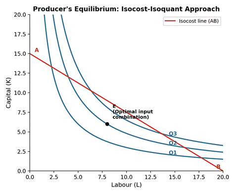
Figure: Point E, where the isocost line AB is tangent to isoquant Q2, is the least-cost combination of labour and capital for that output level.
In the diagram, Q1, Q2 and Q3 are successive isoquants representing increasing levels of output, and AB is the isocost line determined by the firm’s budget and the prevailing input prices. Every point on AB is affordable, but only point E — where AB is tangent to isoquant Q2 — lies on the highest isoquant the firm can reach with that budget. At any other point on AB (e.g., where AB crosses Q1), the firm could produce the same output at lower cost, or produce more output for the same cost, by moving along AB toward E. At E, the slope of the isocost line equals the slope of the isoquant, so the rate at which the market allows the firm to substitute capital for labour (w/r) exactly equals the rate at which the technology allows it to do so (MRTS). This is the firm’s equilibrium — the optimal combination of inputs in the long run, when both labour and capital are variable.
If input prices change (say wages rise relative to the rental of capital), the isocost line becomes steeper and a new tangency point is established further along the isoquant map with more capital and less labour — this traces the firm’s expansion path or factor-substitution behaviour over time.
Q4. Critically analyze pricing decisions under Perfect Competition and under Monopoly.
Pricing behaviour differs fundamentally between these two market structures because of differences in the number of sellers, control over price, nature of the product, and entry conditions. Analysing the two polar cases side by side is useful because most real-world markets — monopolistic competition, oligopoly — can be understood as lying somewhere along the spectrum between them.
Characteristics of Perfect Competition
Perfect competition is defined by a demanding set of theoretical assumptions: a very large number of buyers and sellers, none of whom individually can influence the market price; a completely homogeneous (undifferentiated) product, so buyers are indifferent as to which seller they purchase from; free entry and exit of firms in the long run; perfect information available to all participants about prices and product quality; and perfect mobility of factors of production. While no real market meets every assumption exactly, agricultural commodity markets and some financial markets (e.g., foreign exchange, certain stock markets) approximate it reasonably well.
Pricing Under Perfect Competition
Under perfect competition, no single firm is large enough to influence the market price; each firm is a ‘price taker’ that accepts the price determined by the interaction of industry demand and supply. For an individual firm, therefore, the demand curve is perfectly elastic (horizontal) at the ruling market price, and Price = Average Revenue = Marginal Revenue.
A firm maximises profit at the output where Marginal Cost equals Marginal Revenue (MC = MR), which, since MR = Price here, becomes MC = Price. Additionally, for this to be a genuine profit-maximum (rather than a profit-minimum), the MC curve must be rising at the point of intersection with the price line — the second-order condition of profit maximisation.
Short run: In the short run, at least one input (typically plant/capital) is fixed, so the firm cannot freely enter or exit the industry. Depending on where the given market price sits relative to the firm’s average cost curve, three outcomes are possible: (i) if Price exceeds Average Cost at the profit-maximising output, the firm earns supernormal (abnormal) profit; (ii) if Price equals Average Cost, the firm earns only normal profit (zero economic profit, though accounting profit may still be positive); and (iii) if Price falls between Average Variable Cost and Average Total Cost, the firm incurs a loss but continues operating in the short run because it still covers its variable costs and makes some contribution toward fixed costs — it would only shut down immediately if Price fell below Average Variable Cost, since then every unit produced adds to the loss.
Long run: In the long run, all inputs are variable and firms can freely enter or exit. Supernormal profits earned by existing firms attract new entrants, expanding industry supply and driving the market price down; conversely, losses drive inefficient firms out, contracting supply and pushing price back up. This adjustment continues until price settles at the minimum point of the long-run average cost curve, where Price = MR = MC = AC. At this point every active firm earns only normal profit — just enough to keep it in the industry, but no more — and there is no longer any incentive for further entry or exit. This is the defining long-run pricing outcome of perfect competition: price is entirely determined by cost conditions and demand, and no firm possesses any individual power to set price above the competitive level.
Real-life example: Vegetable and foodgrain markets. The wholesale market (mandi) for a crop such as tomatoes or wheat is one of the closest real-world approximations to perfect competition. Thousands of small farmers sell an essentially homogeneous product, no single farmer’s output is large enough to influence the mandi price, and the price on any given day is set purely by the interaction of aggregate arrivals (supply) and aggregate buyer demand — every farmer simply accepts the ruling price rather than naming their own. When a bumper harvest raises supply, mandi prices for that vegetable fall sharply across the board (sometimes even below cost, forcing farmers to dump produce), and when supply is poor after adverse weather, prices rise sharply for every seller simultaneously — exactly the price-taking behaviour predicted by the model. Because entry into farming a particular crop is relatively easy (a farmer can switch which crop to sow the following season) and there is no meaningful barrier stopping more farmers from growing a profitable crop, high prices/profits in one season typically draw more acreage into that crop the next season, pushing supply up and price back down — the real-world counterpart of the long-run entry mechanism that drives price toward the competitive, normal-profit outcome.
Real-life example: Foreign exchange and stock markets. In highly liquid financial markets, such as the market for a widely traded currency pair or a heavily traded blue-chip stock, no single retail trader can move the price by buying or selling; each trader takes the quoted market price as given, information is disseminated almost instantaneously to all participants through exchanges and news feeds, and entry/exit (opening or closing a position) is essentially frictionless. These features make such markets behave very close to the perfectly competitive ideal, even though the ‘product’ being traded is a financial asset rather than a physical good.
Characteristics of Monopoly
A monopoly is a market with a single seller of a product with no close substitutes, facing significant barriers to entry that prevent competition from emerging — these barriers may be legal (patents, licences), technological (large economies of scale creating a ‘natural monopoly’), or based on control over an essential input or resource. Because the monopolist is the entire industry, there is no distinction between the firm’s demand curve and the market demand curve — it faces the downward-sloping market demand curve directly.
Pricing Under Monopoly
To sell an additional unit, the monopolist must lower price — not just on the marginal unit, but (in a single-price market) on all previous units as well. Consequently, Marginal Revenue is less than Average Revenue (Price) at every output level beyond the first unit, and the MR curve lies below and falls faster than the demand (AR) curve. Mathematically, if demand is P = a − bQ, then Total Revenue = PQ = aQ − bQ², and Marginal Revenue = a − 2bQ, which falls twice as steeply as demand — a relationship visible in the pricing diagram below.
The monopolist maximises profit at the output where MC = MR (as with any firm, since this is the universal profit-maximising rule), but then charges the price read off the demand curve at that output — which is higher than marginal cost. This is the key structural difference from perfect competition: Price exceeds Marginal Cost under monopoly, whereas Price equals Marginal Cost under perfect competition. Because entry is blocked, the monopolist can continue to earn supernormal profits even in the long run; there is no competitive mechanism to erode them, unlike in perfectly competitive markets.
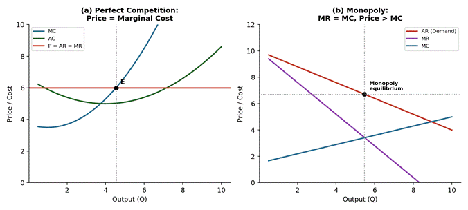
Figure: (a) Under perfect competition the firm is a price taker and equates Price with MC. (b) Under monopoly the firm equates MR with MC but sets Price above MC, restricting output relative to the competitive outcome.
Critical Comparison
| Aspect | Perfect Competition | Monopoly |
| Price-setting power | None — price taker | Full — price maker (subject to demand) |
| Demand curve facing firm | Perfectly elastic (horizontal) | Downward sloping (= market demand) |
| Equilibrium condition | P = MR = MC | MR = MC, but P > MC |
| Long-run profit | Only normal profit (entry/exit) | Can be supernormal (barriers to entry) |
| Output level (for similar cost) | Higher, allocatively efficient (P = MC) | Lower — restricts output to raise price |
| Consumer welfare | Higher (lower price, more output) | Lower (higher price, deadweight loss) |
From a welfare standpoint, perfect competition is often regarded as allocatively efficient because price equals the marginal cost of production, reflecting the true opportunity cost of resources to society. Monopoly pricing, by contrast, restricts output below the competitive level and charges a price above marginal cost, creating a deadweight loss to society — part of consumer surplus is transferred to producer surplus (monopoly profit) and part is simply lost. In practice, most real-world markets lie between these two extremes (monopolistic competition, oligopoly), but the polar cases remain the essential benchmarks for analysing pricing power and its welfare consequences.
Q5. Explain Price Discrimination. Does Price Discrimination exist in the real world? Discuss with reference to any particular product or service.
Meaning of Price Discrimination
Price discrimination refers to the practice of a seller charging different prices to different buyers, or different prices for different units of the same good, for reasons not fully justified by differences in the cost of supplying them. It is typically practised by firms with some degree of monopoly power, since a purely competitive firm has no control over price at all — price discrimination is, in this sense, a natural extension of monopoly (or oligopoly/monopolistic competition) pricing behaviour once the seller recognises that different customers, or different units sold to the same customer, have different price elasticities of demand.
The underlying economic motive is straightforward: a single uniform price forces the seller to leave money on the table — some customers would have paid more than the uniform price (their surplus is ‘given away’), while charging a uniform price high enough to capture that surplus from high-value customers would exclude price-sensitive customers altogether. By separating buyers or units and charging each what they are willing to pay, the seller can increase total revenue and profit beyond what uniform pricing allows, and in some cases can even expand total output and access markets that a single uniform price would leave unserved.
Degrees of Price Discrimination
- First-degree (perfect) price discrimination: The seller charges each individual consumer the maximum price they are willing to pay for each unit, capturing the entire consumer surplus as producer surplus, leaving buyers with no surplus at all. This is rare in pure form but approximated by personalised pricing, bargaining in bazaars and used-car markets, professional fees individually negotiated by doctors or lawyers, and increasingly by online ‘dynamic pricing’ algorithms that use browsing history and purchase data to estimate an individual buyer’s willingness to pay.
- Second-degree price discrimination: The seller charges different prices for different quantities or ‘blocks’ of the same good, without needing to identify individual buyers — for example, bulk discounts, quantity discounts, or tiered/block pricing (e.g., increasing block tariffs for electricity or water, where the per-unit rate is higher above a certain usage threshold, or subscription plans offering a lower per-unit price at higher tiers of usage).
- Third-degree price discrimination: The seller separates buyers into distinct groups based on some identifiable, non-transferable characteristic (age, location, occupation, time of purchase, student status) and charges each group a different price, based on that group’s elasticity of demand — charging a lower price to the more elastic group and a higher price to the less elastic group. This is the most commonly observed form in everyday markets.
The condition determining the profit-maximising price gap between segments under third-degree discrimination follows directly from elasticity: the monopolist sets a lower price in the market segment with higher (more elastic) demand and a higher price in the segment with lower (more inelastic) demand, because raising price in an elastic segment causes a proportionately larger fall in quantity sold (and hence revenue), while raising price in an inelastic segment barely reduces quantity sold, so more revenue can be extracted there without much loss of volume. This is precisely why the concept of price discrimination connects directly back to the elasticity analysis in Question 2 — sellers price-discriminate according to elasticity, targeting higher prices at the segments whose demand is least sensitive to price (i.e., the segments with fewer effective substitutes).
Conditions Necessary for Price Discrimination
For discrimination to be effective and sustainable, several conditions must hold simultaneously:
- Market power: The seller must have some degree of monopoly power (downward-sloping demand curve) — a perfectly competitive firm, facing a horizontal demand curve at the market price, has no scope to charge different prices.
- Identifiable market segmentation: The seller must be able to identify or segment distinct groups of buyers, or distinct units of purchase, with differing price elasticities of demand.
- Prevention of resale (no arbitrage): The seller must be able to prevent buyers in the low-price segment from reselling to buyers in the high-price segment; if resale were easy, arbitrageurs would buy cheap in the low-price market and resell in the high-price market, eroding the price gap until a single price prevailed. This is why price discrimination is far more common in services (which cannot easily be resold, e.g., a haircut, a medical consultation, an airline seat tied to an ID) than in easily transportable physical goods.
- Different price elasticities across segments: The segments must genuinely differ in their responsiveness to price for discrimination to be profitable — if all segments had identical elasticity, there would be no gain from separating them.
Does Price Discrimination Exist in the Real World?
Yes — price discrimination is extremely common and can be observed across many industries, in all three degrees described above. A particularly rich illustration is the airline industry, which exhibits several forms of discrimination simultaneously.
Example: Airline Ticket Pricing. Airlines are a textbook case of third-degree (and increasingly first-degree, algorithmic) price discrimination. Passengers on the very same flight, seated in the very same class of cabin, routinely pay very different fares for what is essentially an identical service (a seat from origin to destination).
- Segmentation by time of booking: Fares rise as the departure date approaches, since last-minute travellers (often business travellers with inelastic demand) are willing to pay more, while early bookers (typically leisure travellers with elastic demand and more flexibility) get lower advance-purchase fares.
- Segmentation by traveller type: Business travellers, who need flexibility and are often reimbursed by employers, are charged much higher fares for flexible, refundable tickets, while leisure travellers accept restrictive, non-refundable, non-changeable fares in exchange for a much lower price — this is a classic Saturday-night-stay type screening device that separates elastic from inelastic demanders.
- Segmentation by group: Discounted fares for students, senior citizens, defence personnel, or children reflect different willingness/ability to pay across demographic groups.
- Dynamic/algorithmic pricing: Airlines use sophisticated revenue-management software that adjusts prices continually based on booking patterns, seat inventory, and even the specific route/day combination, pushing the practice closer to first-degree discrimination as more individual-level data becomes available.
Resale is prevented because airline tickets are typically non-transferable and tied to the passenger’s identity document, which is precisely what makes this form of discrimination sustainable — a passenger who bought a cheap advance fare cannot resell it to a last-minute business traveller.
Further Real-World Examples
Similar examples abound elsewhere in the economy, illustrating each of the three degrees of discrimination:
| Sector/Product | Basis of segmentation | Degree of discrimination |
| Movie theatres | Matinee vs evening show; student/senior discounts | Third-degree |
| Electricity/water utilities | Increasing block tariffs by usage slab | Second-degree |
| Streaming/software subscriptions | Free/basic/premium tiers; student and regional pricing | Second- and third-degree |
| Hospitals and private education | Income-based or category-based fee structures | Third-degree |
| Telecom data plans | Different rates across circles/customer segments | Third-degree |
| E-commerce dynamic pricing | Personalised pricing based on browsing/purchase history | Approaching first-degree |
| Railways (reservation classes) | Sleeper/AC/Tatkal fare differentials on the same route | Second- and third-degree |
Example: Movie Theatre Pricing. A cinema hall charges a lower price for a weekday matinee show than for a weekend evening show, and offers further discounts to students and senior citizens presenting valid identification. The seats and the film are identical; what differs is the willingness to pay of each segment — weekday afternoon audiences (often students, retirees, or those with flexible schedules) have more elastic demand and more substitute activities available, while weekend evening audiences (often working professionals seeking a fixed leisure slot) have less elastic demand. The theatre thus extracts higher revenue from the less price-sensitive segment while still filling seats that would otherwise sit empty during off-peak hours by offering the price-sensitive segment a lower fare — an outcome that can raise both theatre profit and total attendance compared with a single uniform price.
Conclusion
Price discrimination is not merely a theoretical curiosity — it is a pervasive and economically rational strategy used by firms with market power to increase revenue and profit by capturing a larger share of consumer surplus, as vividly illustrated by airline ticket pricing, cinema pricing, utility tariffs, and numerous other everyday examples. While it can raise seller profits and sometimes even expand total output and access to a good or service (by making it accessible to price-sensitive segments who would otherwise not purchase it at all under a single high uniform price), it also raises equity concerns since identical services are sold at different prices to different consumers based purely on their willingness or ability to pay, and it requires firms to invest considerably in market segmentation, screening devices, and (increasingly) data analytics to sustain the practice over time.